7 Appendix: UKTM model & input assumptions
Reading time: 18 minutes
UKTM overview
UK TIMES Model (UKTM) represents the existing energy system in 2010, including the existing infrastructure assets (power generation plants, vehicle stock etc.) across sectors, and flows of energy.
The whole system is represented, from resource extraction, through to primary and secondary fuel production (electricity, hydrogen, biofuels), and finally consumption in the residential, industrial, service, transport and agricultural sectors. This final consumption is used to meet the wide range of energy service demands needed across the economy, such as mobility, heating, and industrial production.
For scenario exercises, projected energy service demands are exogenous inputs into the model. The model then solves by exploring least cost supply-side solutions to meeting those future service demands. The whole system representation allows for the trade-offs between sectors in respect of resource allocation. Demands for energy vectors, such as electricity and hydrogen, are determined endogenously by the model, and are sensitive to changing prices driven by the dynamics of balancing demand and supply.
The other benefit of the whole system representation is that it allows for comprehensive and internally consistent accounting of energy-related greenhouse gases, and includes other key non-energy sources, such as agriculture and land use. This means the model can be used for exploring energy systems that meet climate and energy policy goals.
Structurally, UKTM is a single spatial node model covering the whole of the UK. As such the import and export of energy commodities take place with the rest of the world by combining assumptions of unit cost, and maximum supply levels based on expectations for the markets that these commodities are exchanged on. The model, calibrated to 2010, explores system evolution out to 2060. Time within the model is represented by 16 time-slices (one typical day for each season, split into daytime, evening peak, late evening and night). This structure was determined based on the shape of the electricity demand load in 2010. To find the partial equilibrium, the supply-demand balance has to be found across all different energy commodities, both annually but also at a sub-annual level e.g. for a given time-slice.
The component parts of UKTM are shown in Figure A1.
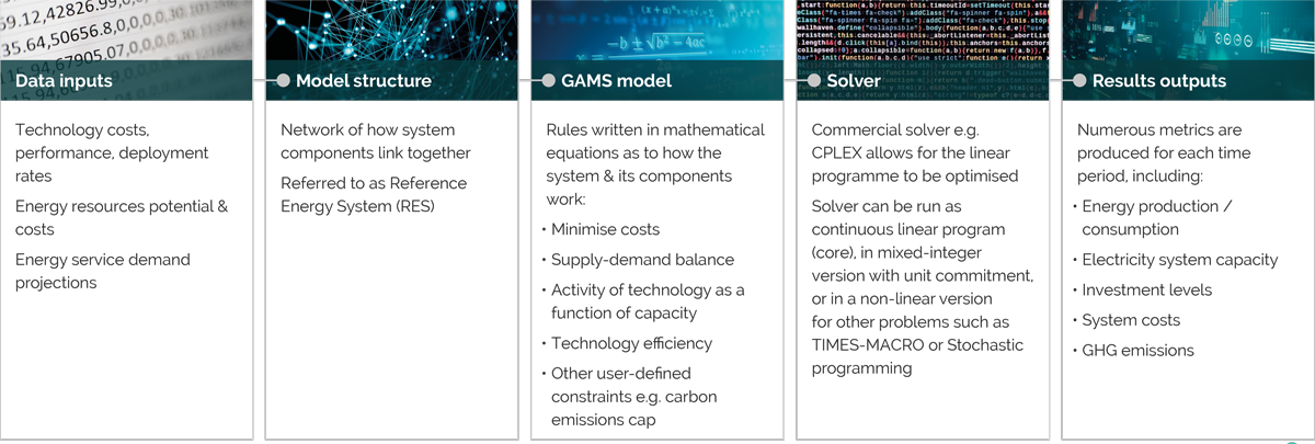
Image text
Data inputs:
- Technology costs, performance, deployment rates
- Energy resources potential & costs
- Energy service demand projections
Model structure:
- Network of how system components link together
- Referred to as Reference Energy System (RES)
GAMS model:
Rules written in mathematical equations as to how the system & its components work:
- Minimise costs
- Supply-demand balance
- Activity of technology as a function of capacity
- Technology efficiency
- Other user-defined constraints e.g. carbon emissions cap
Solver:
- Commercial solver e.g. CPLEX allows for the linear programme to be optimised
- Solver can be run as continuous linear program (core), in mixed-integer version with unit commitment, or in a non-linear version for other problems such as TIMES-MACRO or Stochastic programming
Results outputs:
Numerous metrics are produced for each time period, including:
- Energy production / consumption
- Electricity system capacity
- Investment levels
- System costs
- GHG emissions
TIMES Model equations
The model input assumptions are compiled and used in the linear programme (using GAMS code), in which the rules of the system operation and evolution are defined based on a set of mathematical equations. Below we outline some of the key equations used in the model; the full source code can be found on Github, with full documentation available on the ETSAP website.
In simple terms, an optimisation model such as UKTM will –
- minimise the objective function (total system costs)
- whilst satisfying the energy service demand requirements
- and respecting user-defined system constraints.
The key equations that set the rules of the model LP (linear programming) problem are summarised below.
Objective function (EQ_OBJ). The function is to minimise total discounted system costs.
Where disc is the global discount rate, varom is the variable O&M costs associated with technology activity (ACT), invcost is the capital expenditure associated with new investment (NCAP), discounted using the crf (capital recovery factor), impprice is the price of imports, multiplied by import level (IMP), expprice is the price of exports, multiplied by export level (EXP), and flocost is the cost of other domestic energy commodities (FLO).
Where index y is year, p is process (technology), c is energy commodity, and ts is time segment.
Commodity balance (EQ(l)_COMBAL). This equation ensures that the production of a commodity is equal to its consumption, to balance commodity markets.
Transformation equation (EQ_PTRANS). This establishes the relationship between an input commodity to a technology and an output commodity e.g. technology efficiency.
Where ηɳ is the efficiency factor, and FLOcin and FLOcout represent the input and output commodities of a technology.
Product allocation constraint (EQ(l)_INSHR/OUTSHR). Allows for the control of different commodity shares, where there are more than one input or output commodities into a technology.
Where floshar defines the share of the single commodity (numerator) over the sum of commodities (denominator), or commodity group (index cg).
Activity definition (EQ_ACTFLO). Activity of a technology is a function of the commodity flow, either of inputs but more typically outputs.
Utilisation constraint (EQ_CAPACT). Ensures that the activity of a technology is a function of its capacity.
While the above equations constitute the key set used in the linear programme, a full listing can be found in Loulou et al, pdf (2016) in Table 24. These include specific equations that bound capacity, activity and commodity production, set the rules for the operation of storage technologies, or ensure capacity exceeds demand for a selected commodity in a given time period (often used to ensure a peak margin for electricity systems).
User-defined equations can also be built to provide more control over the model operation. Most are built using the standard LHS form, where the left hand side of the equation includes the variables to be controlled, while the right hand side (RHS) sets the rule, e.g. must be greater than 10% of total generation (share) or less than 50 GW capacity (absolute). Other user constraints are more dynamic in nature e.g. growth constraints that set % changes on the preceding period levels. A number of these constraints are outlined in the next section.
Key model assumptions
A range of assumptions have been incorporated into UKTM from the sector-based analysis; these are described below. We first present the energy service demands, followed by other assumptions added into UKTM, in addition to what is already included in the standard model.
Energy service demands
Energy service demands are provided directly from the sector analyses, as described in section 3.4, and shown in Tables A1 and A2.
For non-energy sectors emissions, land use change and agriculture, we add projections directly in emission terms (CO2e). The projected non-energy agriculture emissions are taken directly from the nutrition analysis (Garvey et al 2021), based on the impact of demand side shifts in diet. Remaining on-farm emissions can be mitigated-based on a marginal abatement cost curves for UK agricultural GHGs provided by Defra. Baseline land use emission projections are taken from BEIS with various reforestation options (e.g. different tree types) available to the model.
| Energy service demand | Ignore | Steer | Shift | Transform | |||||||||
|---|---|---|---|---|---|---|---|---|---|---|---|---|---|
| 2010 | 2020 | 2030 | 2040 | 2050 | 2020 | 2030 | 2040 | 2050 | 2020 | 2030 | 2040 | 2050 | |
| Space heating: Existing cavity walled houses | 1.00 | 0.99 | 0.98 | 0.96 | 0.94 | 0.99 | 0.98 | 0.95 | 0.92 | 0.99 | 0.98 | 0.95 | 0.91 |
| Space heating: Existing solid walled houses | 1.00 | 0.99 | 0.98 | 0.96 | 0.94 | 0.99 | 0.98 | 0.96 | 0.93 | 0.99 | 0.98 | 0.96 | 0.92 |
| Space heating: Existing cavity walled flats | 1.00 | 0.99 | 0.98 | 0.94 | 0.91 | 0.99 | 0.98 | 0.93 | 0.88 | 0.99 | 0.98 | 0.94 | 0.87 |
| Space heating: Existing solid walled flats | 1.00 | 0.99 | 0.98 | 0.94 | 0.91 | 0.99 | 0.98 | 0.94 | 0.88 | 0.99 | 0.98 | 0.94 | 0.87 |
| Space heating: New houses | 1.00 | 23.20 | 49.02 | 70.50 | 93.24 | 23.20 | 49.02 | 68.80 | 92.63 | 23.20 | 49.02 | 49.30 | 49.72 |
| Water heating: Existing cavity walled houses | 1.00 | 0.99 | 0.98 | 1.00 | 1.01 | 0.99 | 0.98 | 1.00 | 1.01 | 0.99 | 0.98 | 1.00 | 1.00 |
| Water heating: Existing solid walled houses | 1.00 | 0.99 | 0.98 | 0.99 | 0.99 | 0.99 | 0.98 | 0.99 | 0.99 | 0.99 | 0.98 | 0.98 | 0.98 |
| Water heating: Existing cavity walled flats | 1.00 | 0.99 | 0.98 | 0.99 | 0.99 | 0.99 | 0.98 | 0.99 | 0.98 | 0.99 | 0.98 | 0.99 | 0.98 |
| Water heating: Existing solid walled flats | 1.00 | 0.99 | 0.98 | 0.98 | 0.97 | 0.99 | 0.98 | 0.98 | 0.97 | 0.99 | 0.98 | 0.97 | 0.96 |
| Water heating: New houses | 1.00 | 10.13 | 21.40 | 21.72 | 22.04 | 10.13 | 21.40 | 23.78 | 26.64 | 10.13 | 21.40 | 21.52 | 21.70 |
| Lighting | 1.00 | 1.04 | 1.09 | 1.12 | 1.14 | 1.04 | 1.09 | 1.12 | 1.14 | 1.04 | 1.09 | 0.93 | 0.83 |
| Refrigerators | 1.00 | 1.04 | 1.09 | 1.12 | 1.14 | 1.04 | 1.09 | 1.12 | 1.14 | 1.04 | 1.09 | 1.09 | 1.09 |
| Freezers | 1.00 | 1.04 | 1.09 | 1.12 | 1.14 | 1.04 | 1.09 | 1.12 | 1.14 | 1.04 | 1.09 | 1.09 | 1.09 |
| Wet appliances | 1.00 | 1.04 | 1.09 | 1.12 | 1.14 | 1.04 | 1.09 | 1.12 | 1.14 | 1.04 | 1.09 | 0.93 | 0.93 |
| Consumer electronics | 1.00 | 1.04 | 1.07 | 1.09 | 1.11 | 1.04 | 1.07 | 1.09 | 1.11 | 1.04 | 1.07 | 0.84 | 0.75 |
| Computers | 1.00 | 1.04 | 1.07 | 1.09 | 1.11 | 1.04 | 1.07 | 1.09 | 1.11 | 1.04 | 1.07 | 0.84 | 0.75 |
| Cooking: Other appliances | 1.00 | 1.04 | 1.09 | 1.12 | 1.14 | 1.04 | 1.09 | 1.12 | 1.14 | 1.04 | 1.09 | 1.04 | 1.04 |
| Cooking: Hobs | 1.00 | 1.04 | 1.09 | 1.12 | 1.14 | 1.04 | 1.09 | 1.12 | 1.14 | 1.04 | 1.09 | 1.04 | 1.04 |
| Cooking: Ovens | 1.00 | 1.04 | 1.09 | 1.12 | 1.14 | 1.04 | 1.09 | 1.12 | 1.14 | 1.04 | 1.09 | 1.04 | 1.04 |
| Cooling | 1.00 | 1.70 | 2.46 | 3.28 | 4.15 | 1.70 | 2.46 | 3.28 | 4.15 | 1.70 | 2.46 | 3.12 | 3.74 |
| Other | 1.00 | 1.04 | 1.09 | 1.12 | 1.14 | 1.04 | 1.09 | 1.12 | 1.14 | 1.04 | 1.09 | 1.09 | 1.09 |
| Energy service demand | Ignore | Steer | Shift | Transform | |||||||||
|---|---|---|---|---|---|---|---|---|---|---|---|---|---|
| 2010 | 2020 | 2030 | 2040 | 2050 | 2020 | 2030 | 2040 | 2050 | 2020 | 2030 | 2040 | 2050 | |
| Space heating: Low consumption buildings | 1.00 | 0.98 | 1.03 | 1.09 | 1.15 | 0.98 | 1.02 | 1.06 | 1.10 | 0.98 | 0.98 | 0.98 | 0.99 |
| Water heating: Low consumption buildings | 1.00 | 0.98 | 1.03 | 1.09 | 1.15 | 0.98 | 1.02 | 1.06 | 1.10 | 0.98 | 0.98 | 0.98 | 0.99 |
| Space heating: High consumption buildings | 1.00 | 0.98 | 1.03 | 1.09 | 1.15 | 0.98 | 1.02 | 1.06 | 1.10 | 0.98 | 0.98 | 0.98 | 0.99 |
| Water heating: High consumption buildings | 1.00 | 0.98 | 1.03 | 1.09 | 1.15 | 0.98 | 1.02 | 1.06 | 1.10 | 0.98 | 0.98 | 0.98 | 0.99 |
| Cooling: High consumption buildings | 1.00 | 0.98 | 1.03 | 1.09 | 1.15 | 0.98 | 1.02 | 1.06 | 1.10 | 0.98 | 0.98 | 0.98 | 0.99 |
| Lighting: Offices | 1.00 | 0.98 | 1.03 | 1.09 | 1.15 | 0.98 | 1.02 | 1.06 | 1.10 | 0.98 | 0.98 | 0.98 | 0.99 |
| Lighting: Other | 1.00 | 0.98 | 1.03 | 1.09 | 1.15 | 0.98 | 1.02 | 1.06 | 1.10 | 0.98 | 0.98 | 0.98 | 0.99 |
| Computing | 1.00 | 0.98 | 1.03 | 1.09 | 1.15 | 0.98 | 1.02 | 1.06 | 1.10 | 0.98 | 0.98 | 0.98 | 0.99 |
| Cooking | 1.00 | 0.98 | 1.03 | 1.09 | 1.15 | 0.98 | 1.02 | 1.06 | 1.10 | 0.98 | 0.98 | 0.98 | 0.99 |
| Refrigeration | 1.00 | 0.98 | 1.03 | 1.09 | 1.15 | 0.98 | 1.02 | 1.06 | 1.10 | 0.98 | 0.98 | 0.98 | 0.99 |
| Other | 1.00 | 0.98 | 1.03 | 1.09 | 1.15 | 0.98 | 1.02 | 1.06 | 1.10 | 0.98 | 0.98 | 0.98 | 0.99 |
| Energy service demand | Ignore | Steer | Shift | Transform | |||||||||
|---|---|---|---|---|---|---|---|---|---|---|---|---|---|
| 2010 | 2020 | 2030 | 2040 | 2050 | 2020 | 2030 | 2040 | 2050 | 2020 | 2030 | 2040 | 2050 | |
| Passenger cars | 1.00 | 1.06 | 1.10 | 1.13 | 1.15 | 1.06 | 1.09 | 0.93 | 0.76 | 1.06 | 1.08 | 0.79 | 0.50 |
| Two wheelers | 1.00 | 1.05 | 1.05 | 1.07 | 1.09 | 1.05 | 1.05 | 2.55 | 4.08 | 1.05 | 1.03 | 4.25 | 7.25 |
| Buses | 1.00 | 0.94 | 0.82 | 0.84 | 0.85 | 0.94 | 0.81 | 1.43 | 2.07 | 0.94 | 0.80 | 1.66 | 2.52 |
| LGVs | 1.00 | 1.17 | 1.35 | 1.50 | 1.64 | 1.17 | 1.35 | 1.37 | 1.36 | 1.17 | 1.35 | 1.32 | 1.24 |
| HGVS: Rigid | 1.00 | 1.06 | 1.11 | 1.17 | 1.23 | 1.06 | 1.11 | 1.07 | 1.02 | 1.06 | 1.11 | 1.03 | 0.93 |
| HGVS: Articulated | 1.00 | 1.08 | 1.13 | 1.19 | 1.26 | 1.08 | 1.13 | 1.09 | 1.04 | 1.08 | 1.13 | 1.05 | 0.95 |
| Rail: Passenger | 1.00 | 1.09 | 1.08 | 1.10 | 1.12 | 1.09 | 1.08 | 1.34 | 1.60 | 1.09 | 1.06 | 1.44 | 1.78 |
| Rail: Freight | 1.00 | 1.09 | 1.15 | 1.22 | 1.30 | 1.09 | 1.15 | 1.22 | 1.30 | 1.09 | 1.15 | 1.23 | 1.30 |
| Aviation: Domestic | 1.00 | 0.94 | 0.65 | 0.89 | 0.92 | 0.94 | 0.65 | 0.75 | 0.74 | 0.94 | 0.65 | 0.65 | 0.62 |
| Aviation: International | 1.00 | 1.09 | 0.57 | 1.07 | 1.13 | 1.09 | 0.57 | 0.85 | 0.84 | 1.09 | 0.57 | 0.65 | 0.62 |
| Shipping: Domestic | 1.00 | 1.00 | 0.93 | 0.88 | 0.76 | 1.00 | 0.93 | 0.88 | 0.76 | 1.00 | 0.93 | 0.88 | 0.76 |
| Shipping: International | 1.00 | 1.09 | 1.09 | 1.09 | 1.14 | 1.09 | 1.09 | 1.09 | 1.14 | 1.09 | 1.09 | 1.09 | 1.14 |
| Energy service demand | Ignore | Steer | Shift | Transform | |||||||||
|---|---|---|---|---|---|---|---|---|---|---|---|---|---|
| 2010 | 2020 | 2030 | 2040 | 2050 | 2020 | 2030 | 2040 | 2050 | 2020 | 2030 | 2040 | 2050 | |
| Iron and steel | 1.00 | 1.12 | 0.76 | 0.74 | 0.73 | 1.12 | 0.76 | 0.71 | 0.67 | 1.12 | 0.76 | 0.64 | 0.55 |
| Cement | 1.00 | 0.88 | 0.94 | 0.99 | 1.05 | 0.88 | 0.94 | 0.98 | 1.02 | 0.88 | 0.94 | 0.59 | 0.61 |
| Non-metallic minerals | 1.00 | 0.88 | 0.94 | 0.98 | 1.03 | 0.88 | 0.94 | 0.97 | 1.00 | 0.88 | 0.94 | 0.53 | 0.54 |
| Paper | 1.00 | 0.93 | 0.83 | 0.76 | 0.70 | 0.93 | 0.83 | 0.74 | 0.67 | 0.93 | 0.83 | 0.73 | 0.63 |
| Chemicals: HVC | 1.00 | 0.88 | 0.83 | 0.80 | 0.80 | 0.88 | 0.83 | 0.80 | 0.78 | 0.88 | 0.83 | 0.79 | 0.76 |
| Chemicals: Ammonia | 1.00 | 0.88 | 0.83 | 0.80 | 0.80 | 0.88 | 0.83 | 0.80 | 0.79 | 0.88 | 0.83 | 0.79 | 0.77 |
| Chemicals: Other | 1.00 | 0.88 | 0.83 | 0.80 | 0.80 | 0.88 | 0.83 | 0.80 | 0.79 | 0.88 | 0.83 | 0.80 | 0.79 |
| Non-ferrous metals | 1.00 | 0.77 | 0.78 | 0.71 | 0.66 | 0.77 | 0.78 | 0.70 | 0.64 | 0.77 | 0.78 | 0.69 | 0.62 |
| Food and drink | 1.00 | 1.06 | 1.08 | 1.10 | 1.11 | 1.06 | 1.08 | 1.09 | 1.10 | 1.06 | 1.08 | 1.09 | 1.09 |
| Other industry | 1.00 | 0.99 | 1.00 | 1.01 | 1.01 | 0.99 | 1.00 | 0.99 | 0.98 | 0.99 | 1.00 | 0.98 | 0.94 |
| Chemicals: Non-energy | 1.00 | 0.88 | 0.83 | 0.80 | 0.80 | 0.88 | 0.83 | 0.80 | 0.79 | 0.88 | 0.83 | 0.80 | 0.79 |
| Energy service demand | Ignore | Steer | Shift | Transform | |||||||||
|---|---|---|---|---|---|---|---|---|---|---|---|---|---|
| 2010 | 2020 | 2030 | 2040 | 2050 | 2020 | 2030 | 2040 | 2050 | 2020 | 2030 | 2040 | 2050 | |
| Transport | 1.00 | 1.08 | 1.09 | 1.09 | 1.09 | 1.08 | 1.09 | 1.09 | 1.07 | 1.08 | 1.09 | 1.09 | 1.06 |
| Electricity | 1.00 | 1.08 | 1.09 | 1.09 | 1.09 | 1.08 | 1.09 | 1.09 | 1.07 | 1.08 | 1.09 | 1.09 | 1.06 |
| Heat | 1.00 | 1.08 | 1.09 | 1.09 | 1.09 | 1.08 | 1.09 | 1.09 | 1.07 | 1.08 | 1.09 | 1.09 | 1.06 |
Mobility
For mobility, the differences between scenarios are all driven by changes in energy service demands. In respect of meeting those demands, all technology-based assumptions are the same across scenarios. For road transport, all vehicle efficiency information has been aligned with the Transport Energy and Air pollution Model (TEAM) model assumptions.
| Assumption | Description | Value | |||
|---|---|---|---|---|---|
| Road transport | |||||
| Restrict sales of ICE cars | Year when ban into force on car sales that are not zero carbon based on tail pipe emissions | 2035 | |||
| Battery electric vehicles (BEV) costs | Update of BEV costs (£2010/vehicle) | Year | 2030 | 2040 | 2050 |
| Car | 15,900 | 14,300 | 13,000 | ||
| Bus | 121,000 | 110,000 | 100,000 | ||
| Biofuel use | Maximum share of biofuels in ICEs | 20% | |||
| Constraints: upper limits on vehicle shares | Diesel cars Electric buses Electric rail (freight and passenger) HGV hybrids (pre-2030, unconstrained after) Car PHEVs (pre-2025, unconstrained after) ULEV buses sales (battery electric and H2) unconstrained after | 78%, 80%, 82%, 2%, 58%, 80% | |||
| Annual growth constraints | Electric vehicles All other low carbon technologies | 30%, 25% | |||
| Shipping and aviation | |||||
| Biokerosene use | Biokerosene maximum share by 2050 | 35% | |||
| Ammonia use | Maximum level of ammonia use in shipping by 2050 | 70% | |||
Shelter
| Assumption | Description | Steer | Shift | Transform |
|---|---|---|---|---|
| Building retrofit (Maximum technical potential) | Building retrofit related energy savings are accounted for in the sectoral analysis using the National Housing model (NHM). The corresponding MTP is therefore removed from UKTM. | 0 TWh | ||
| Use of gas for cooking | The minimum level of gas-based cooking in the residential sector is lowered to appropriate levels. | From 35% in 2010 to 0% by 2030 | ||
| Use of gas boilers | The installation of gas boilers in new build dwellings is phased out by a given target year. This includes all fossil boilers (e.g. kerosene) and also applies to district heating for new build. | 2030 | 2020 | 2020 |
| Hybrid boiler fuel use | Hybrid boiler systems – i.e. systems that include a combined boiler and HP system – are assumed to use either hydrogen or clean syngas from a given year onwards. This applies to new and existing dwellings. | 2030 | ||
| HP efficiency alignment | Heat pump coefficients of performance (CoP) used in UKTM are aligned with values assumed in the NHM. CoP values detailed for ASHP and GSHP in existing and new dwellings as well as for DH. All adjustments are made to align by 2030. | DH HP 3.5 Ex ASHP 2.51 Nw ASHP 2.89 Ex GSHP 3.04 Nw GSHP 3.5 | ||
| HP availability | Year from which HP technologies are made available in new and existing dwellings to align dynamics of technology change with NHM assumptions. This combines both ground and air source HP systems. | Ex 2030 Nw 2035 | Ex 2025 Nw ASHP 2020 Nw GSHP 2025 | Ex 2025 Nw |
| HP rollout | S-curve based restriction to HP MTP (Year, % share). MTP calculated assuming 5kW system per household and 1.5 million installations p.a. | 2025, 10 2030, 40 2035, 70 2045, 80 |
2025, 20 2030, 50 2035, 85 2045, 100 |
2025, 15 2030, 60 2035, 100 2045, 100 |
| Gas boiler efficiency | Values included in UKTM are adjusted to values that align in principle with the NHM. Adjustment made by 2030 in all cases and maintain the relative difference across the wider range of technology options included in UKTM. Values declared per Sector, boiler input, and value. | DH, NG and H2, 95% DH, BM, 90% HS, NG, 89% HS, oil, 89% HS, H2, 89% HS, BM, 79% |
||
| Solar hot water | Share of hot water provided through solar thermal systems. This applies to the combined use of household and district-based solutions. | 25% | 30% | – |
| Low energy lighting (LED – light emitting diode) | Non-LED lighting is phased out as an option by a target year in line with NHM assumptions. | 2025 | ||
| Limits to micro combined heat and power (CHP) | Not used in the NHM, micro-CHP is left as an option in UKTM but constrained to start later and grow at a limited pace. Start year and annual growth rate cover total micro-CHP capacity in all dwellings | 2030, 10% p.a. | ||
| Biomass use | Not used in the NHM, biomass is kept as an option in UKTM but constrained by limiting resource input to the sector to an assumed MTP. | 2015 – 10PJ/a 2050 – 20 PJ/a Linear increase |
||
| Limit to DH | Maximum use of district heat in supplying residential demand for heat. | 34% | ||
| Use of wet heating systems | Minimum share of wet heating systems in residential buildings | HC 94%; HS 94%; FC 67%; FS; 82%; NH 87%* | ||
| HP penetration | Maximum share of residential buildings compatible with using a HP due to space constraints. | HC 82%; HS 79%; FC 13%; FS; 10%; NH 68%* | ||
| Natural gas connections | Maximum limit on gas connections in the residential sector accounting for rural locations. | HC 93%; HS 89%; FC 63%; FS; 83%; NH 90%* | ||
| *HC: cavity insulated house; HS: solid wall insulated house; FC: cavity wall insulated flat; FS: solid wall insulated flat; NH: new home; Ex: Existing dwellings; Nw: New dwellings; DH – district heating; HP: heat pump; ASHP: air source heat pump; GSHP: ground source heat pump; WSHP: water source heat pump | ||||
Non-domestic
| Assumption | Description | Steer | Shift | Transform |
|---|---|---|---|---|
| Annual technology growth rate | Upper limit on annual increase in quantity of heat supplied using selected technologies ((ASHP, GSHP, WSHP, biomass boilers) | 10%/a | ||
| Energy saving through building retrofit | Gradual increase in total energy savings available through building retrofit measures as roll-out capacity is assumed to increase with larger workforce and supply chains. Values reported below for individual measures include potential in [2020;2050] in TWh for high (H) and low (L) energy consuming buildings. | |||
| Efficient hot water delivery | L [0.01; 0.15] H [0.01; 0.22] |
L [0.03; 0.22] H [0.04; 0.35] |
||
| Building instrumentation and carbon & energy management | L [0.5; 7.5] H [0.88; 14.0] |
L [1.26; 11.44] H [2.01; 18.3] |
||
| Improved cool storage, cooling & ventilation | H [0.01; 0.13] | H [0.05; 0.42] | ||
| Improved efficiency of small appliances | – | – | L&H [0.04; 0.34] | |
| Heat pump CoP | Annual per-cent increase in heat pump CoP. Increase is applied to existing values in UKTM. It is capped based on the number of years it takes to reach full roll-out (saturation) | 1%/a | ||
| cap 3.51 | cap 3.47 | cap 3.57 | ||
| Hydrogen cooking availability, | Option for hydrogen cooking adjusted for consistency – avoiding its adoption independently of hydrogen heating in buildings. | Option removed | ||
Materials and products
| Assumption | Description | Outcome |
|---|---|---|
| CCS deployment | Limit on CCS in industry sectors such as cement | 2030 |
| Steel production share | Upper limit on the share of steel that can be produced by electric arc furnaces | 55% |
| Biomass use | Upper limits on fuel shares in selected industry subsectors | 15% |
| Gas consumption | Minimum shares of gas use for combustion removed from specific sectors | – |
Electricity
| Assumption | Description | Steer | Shift | Transform |
|---|---|---|---|---|
| Nuclear capacity limit | Cumulative lower and upper limit on fleet capacity by 2050 | Upper limit: 18 GW (Price et al., 2018) Lower limit: 3.2 GW (existing fleet is retired and no new build beyond Hinkley C) |
||
| New nuclear capacity growth rat | Limit on the build rate of new nuclear power | 3 GW (one Hinkley C sized plant) per 5 yrs | ||
| Existing nuclear retirement | All existing plant retired by 2040 | – | ||
| Coal phase-out | Coal generation phase-out by 2025, as per UK policy | All | ||
| Variable renewables capacity growth rates | Annual capacity growth rate assumptions for solar PV and wind. For PV and onshore the absolute rates are slightly more ambitious than the historical peak deployment. For offshore, this assumes peak build rates are sufficient to achieve the Offshore Wind Sector Deal’s 40 GW target by 2030.(Vaughan, 2018b; Vaughan, 2018a). | Solar: 15% per yr and 4.5 GW/yr Wind: 20% per yr and 3 GW/yr each for onshore and offshore wind. |
||
| Offshore Wind Sector Deal | The Offshore Wind Sector Deal target of 40 GW by 2030 is achieved. | All | ||
| Storage (grid electricity) capacity growth rates | Annual capacity growth rate assumptions for all storage technologies combined. | 10% per yr and 5 GW/yr in 2025, rising to 10, 15 and 20 GW/yr by 2030, 2035 and 2050 respectively. | ||
| Annual net interconnector flow | Annual net imports limited to a share of total generation | 5% | ||
| Variable renewable capex | Capex assumptions for solar PV, on and offshore wind (£2010/kW). | 2030 | 2040 | 2050 |
| PV: 330 | 247 | 208 | ||
| Onshore: 770 | 720 | 697 | ||
| Offshore: 1207 (BEIS, 2019a) | 1038 | 1038 | ||
| Total new build capacity limit | The annual rate at which the power system can deploy new capacity in GW/yr | 2030 | 2040 | 2050 |
| 20 | 20 | 30 | ||
Bioenergy, carbon dioxide removal and CCS
| Assumption | Description | Steer | Shift | Transform |
|---|---|---|---|---|
| Bioenergy availability | Levels of biomass output available from domestic and international sources. These levels define the amount of energy available in TWh per annum from different biomass feedstocks. Levels are derived from the CCC 2018 report on biomass availability applying their “Global governance and innovation” scenario. 2050 limits are listed below (CCC, 2018a). | |||
| Imported solid biomass | 102 TWh/a | |||
| Imported liquid biofuels | 53 TWh/a | |||
| Domestic solid biomass | 50 TWh/a | |||
| Domestic agricultural and forestry residues | 67 TWh/a | |||
| Domestic wastes & residues | 28.3 TWh/a | |||
| CCS availability | Year from which commercial scale CCS deployment is permitted | 2030 | ||
| BECCS deployment limits | Direct limits on BECCS sequestration to constrain the model to only what it needs, so that BECCS becomes an option of last resort | No limit imposed | 37 MtCO2 | 0 MtCO2 |
| BECCS emission credit | Due to feedstock sustainability concerns, percentage of CO2 generated available for negative emission credit. | 70% | ||
| DAC availability | Deployment potential of DAC | No limit | 0 MtCO2 | 0 MtCO2 |
| Forestry planting rates | Upper limit on planting rates in ha/yr for biodiversity and energy crops. Rates are applied separately to both classes and are available from 2023. | 9,200 | 50,000 | 100,000 |
Additional results from UKTM modelling
Figure A2 shows the energy demand reductions in the Steer and LED cases (Shift and Transform) by sector. For buildings, this is largely driven by electrification but also much lower new build rates in the Transform cases.
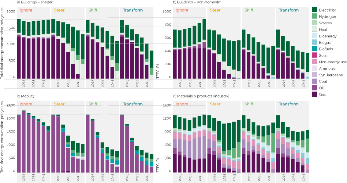
In transport, large reductions result from electrification – but also large reductions in the level of passenger mobility in the LED cases. Industry sees decarbonisation of the energy mix through a range of energy vectors, including hydrogen (green bars) plus resource efficiency gains in the LED cases.
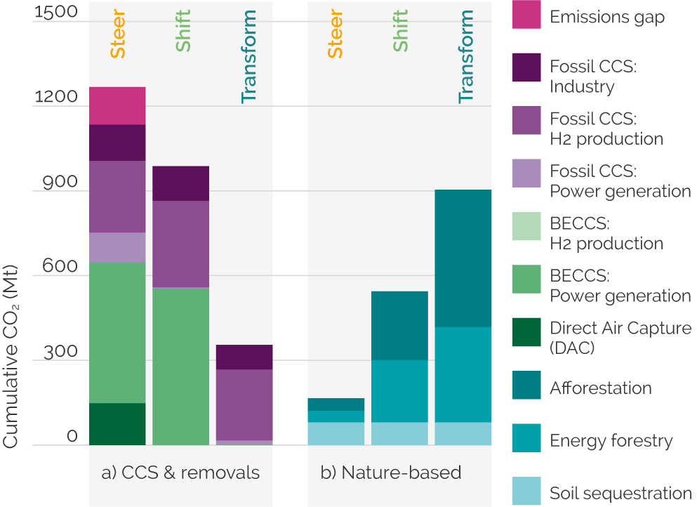
Figure A3 shows the cumulative sequestration from different options in the model, with Steer dominated by engineered removals and CCS, while LED scenarios have a much higher level of nature-based solutions, through types of forestry and soil management.
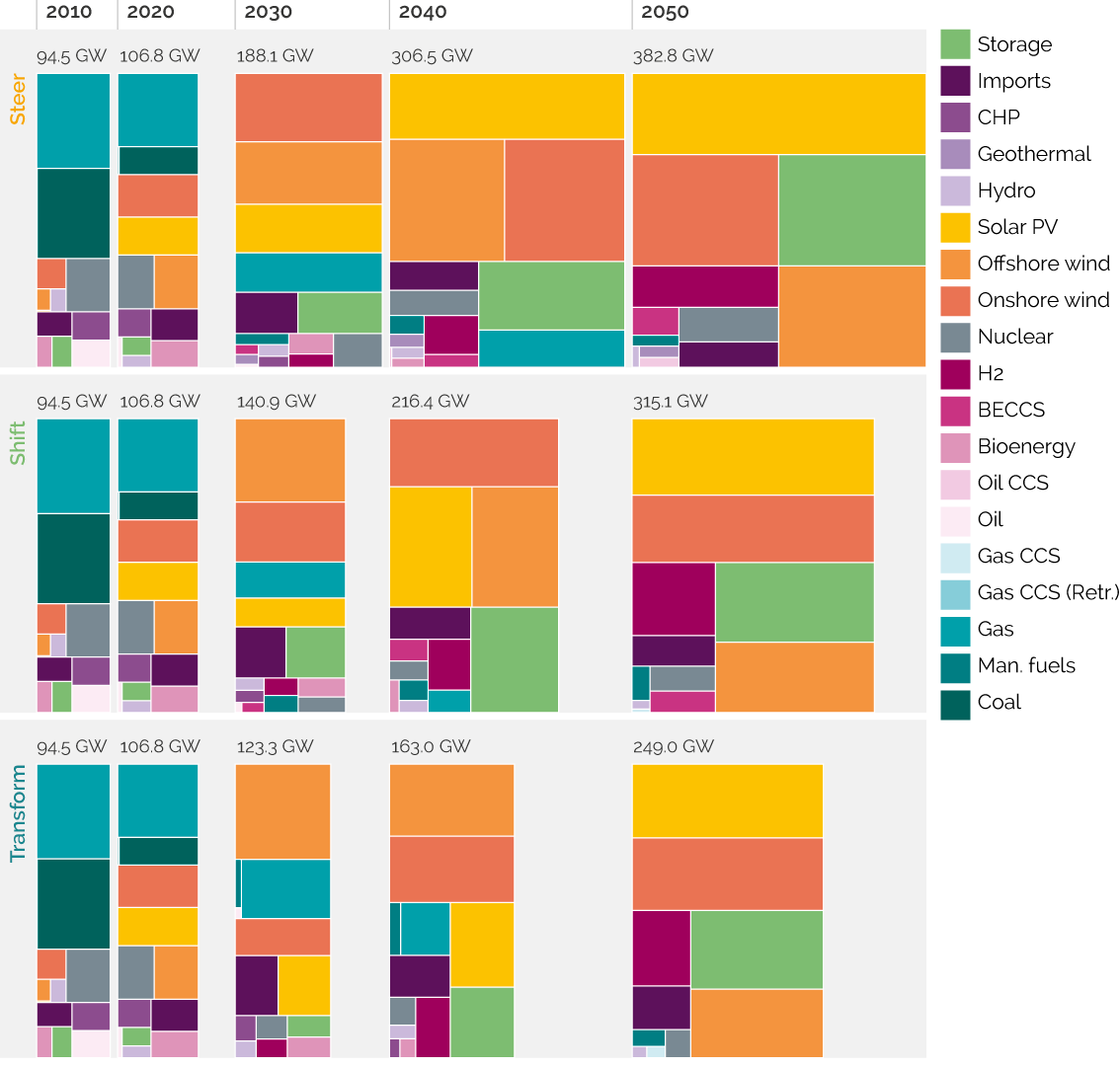
As implied by the power sector generation trajectories in Figure A4, the system capacity levels are much larger in Steer demand compared to the LED cases. This is expected as higher shares of renewable generation (orange and yellow blocks) come online with lower capacity factors. This also requires higher levels of storage (lime green block), with 73 GW in 2050 in the Steer demand case, compared to 46 GW in Transform.
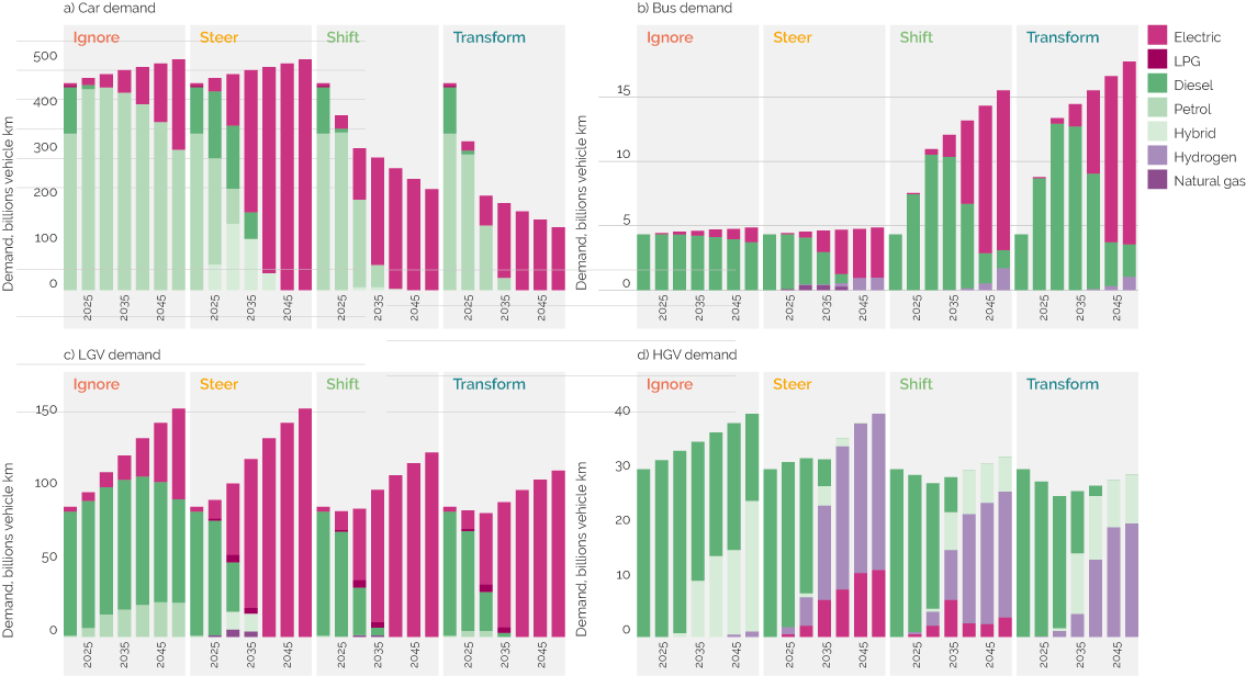
The road transport sector mobility demands are shown below, and the evolution of technology type that meets those demands over time. For cars and LGVs, this means as strong push towards electrification; this also occurs in the Ignore case as EVs become increasingly competitive due to the global shift in manufacturing, irrespective of domestic climate policy.
The level of EVs deployed to meet passenger car demand is massively reduced in the LED cases, compared to the Steer case, which would have huge implications for reducing charging infrastructure, road capacity, and other impacts associated with vehicles (congestion, accidents etc). HGV mobility demand sees a transition towards hydrogen, although a much stronger push towards electrification could be seen under stronger battery cost reductions.
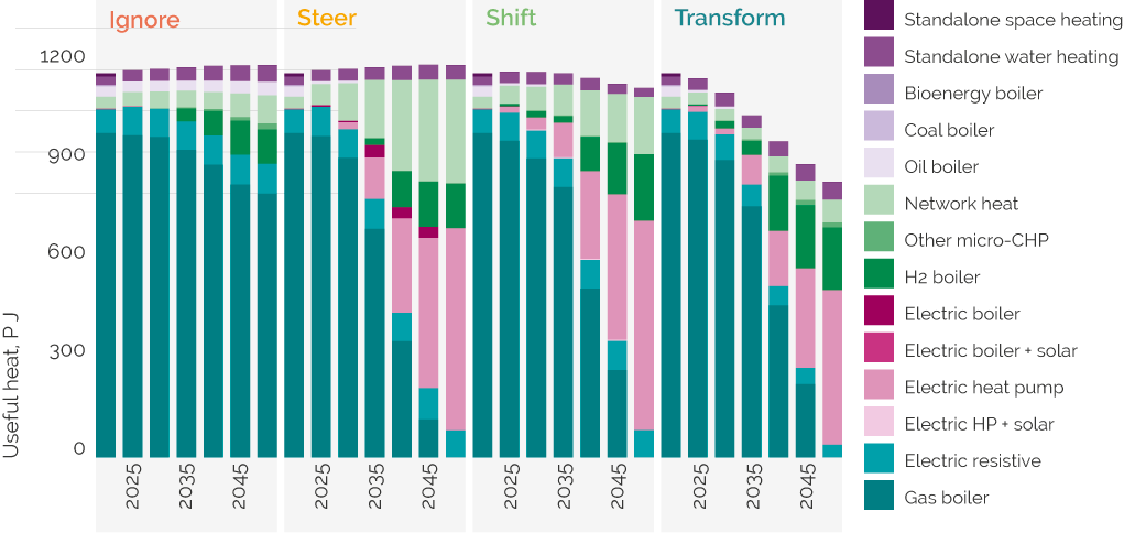
Heat provision in the residential sector is shown in Figure A6, with the impact of retrofit measures taken into account. The strong reduction in energy services in Transform reflects stronger ambition in retrofit plus very low levels of new build. In the main, the pathways show strong heat pump deployment, with smaller shares for heat networks and hydrogen-based systems in specific localities.
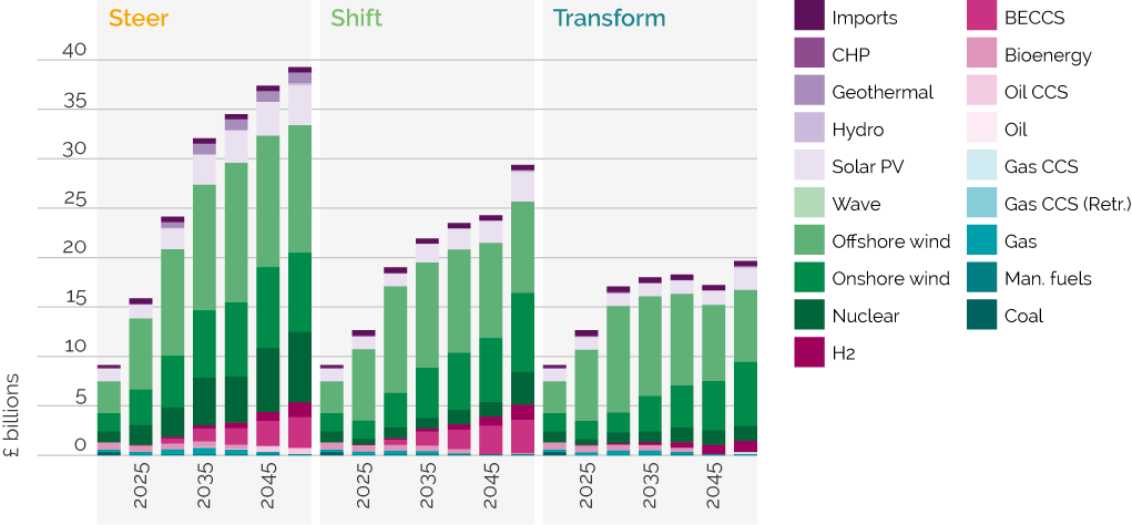
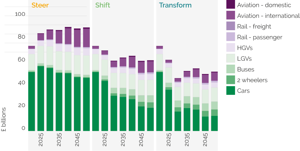
Investment in the power sector across the scenarios highlights the increased levels for low carbon generation. However, this is significantly lower for the LED cases, which require much lower levels of capacity on the system.
The lower levels of capacity requirement are seen across all sectors, not just power generation. The levels of investment across the transport sector decrease dramatically under both LED scenarios, in the main driven by reduced levels of car ownership.